1. Hide content with outlines

For a very quick way to hide certain contents, look no further than the outline option! Select the data you want to hide, then click on the Data ribbon, then go to the far-right to Outline and select Group.

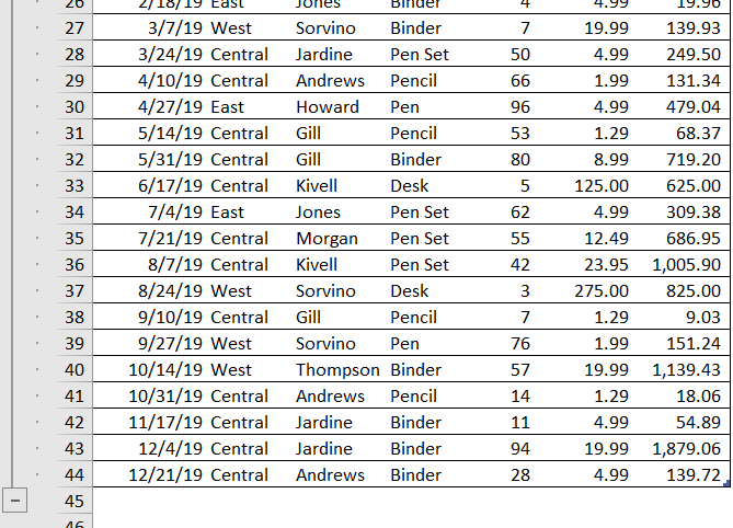
The data you selected will now appear a little different—notice that minus sign on row 45? Clicking on it will hide everything in that bracket automatically!

2. Find out which cells contain formulas

Imagine you were just handed a new sheet, and need to know where exactly all the formulas used are—both so you can make sure they’re right, and change them if you need to.

One way to do this is hitting Ctrl+`—that ` symbol is what many multi-lingual speakers will recognize as a grave accent (used, for instance, like this: à), and its position in the keyboard depends on which type of keyboard you’re using. For American-based ones, it’s usually to the left of the 1 key.

Another way is to select all cells containing formulas. Pres F5, and on the pop-up, click Special and toggle Formulas, hit enter, and that’s it!

3. You can run simple video games

We’ve talked about how Visual Basic can improve and add on functionalities to Excel and other Office products. But did you know some very creative people out there used it to create games that run in Excel?

4. Hide Items through Cell Formatting

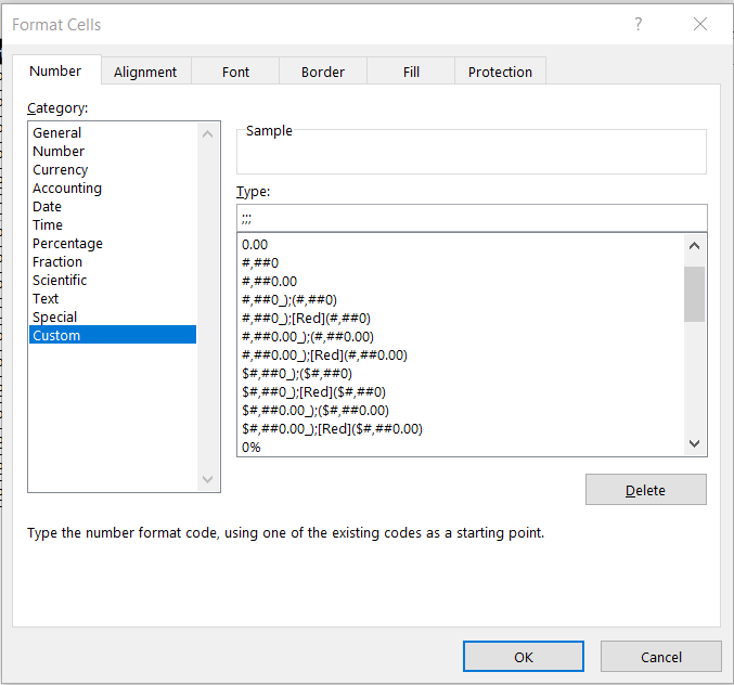
Sometimes, you don’t want to hand out a worksheet with all the data you used, especially when it involved sensitive data. You can do it with outlines, or with cell formatting. To hide a cell through formatting, column, or row, just select it and go to Home->Font->Open Format Cells->Custom and under “Type”, go ahead and enter “;;;” (no quotations). This will leave the chosen cells blank until you re-format them again.

Another option is to go to “Protection” in the Format Cells tab and check the “hidden” box—but that option will only work when you lock your Excel sheet.

5. View Multiple Worksheets from your Workbook

If you need to compare two different worksheets in the same book, there’s an option for that!

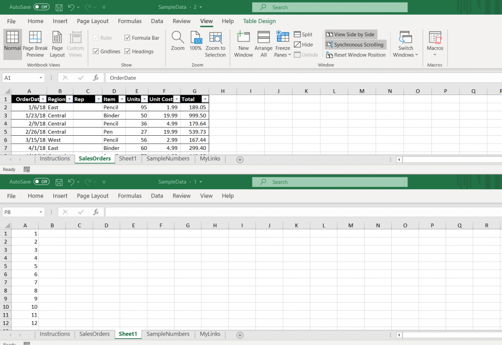
Go in the View tab, and click on Window->New Window. Then again on View, click on View side-by-side and voilá! You can even scroll both at the same time (or not!) with the Synchronous Scrolling option.

6. Solve Mathematical Problems

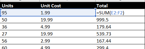
This isn’t really a feature most people don’t know about, but it’s one they might not use often. So if you find that going back and forth between Excel and your Calculator is too much of a bother—well, you don’t have to! Let Excel handle all the basic math through its simple formulas.

7. Get Geographical and Stock Data

You can now add and get Geographical and Stock data in this relatively new Excell feature! And it’s simple to do it too! For Stocks, Just type some text into a cell, (say, “Apple”), go to the Data Tab, and click on Stocks—give it some seconds for Excel to fetch the data, and Apple’s current Stock price will show up in that cell! For Geographic data type a country, province, territory, or city, select the cell, go to the Data tab and click on Geography.

This only works, however, if there’s an online match for your input.

8. Freeze Panes

Ever found yourself scrolling up and down to find a specific piece of data you need for comparison or other purposes? Then this feature is for you! Select the rows and/or columns you want to freeze, then go to the View tab, select Freeze Panes, click on it, and you’re done!

9. Double Clicking

There’s a chance you’ve noticed Excel exhibits different behaviors depending on where you do a double click. Double-clicking up top on the column separator, for instance, will resize the column to fit the data within; if you double-click on the cell border of the first cell in a given row or column, it will snap you to the last cell in the series; and if you have data that follows a pattern in increases or decreases (say, assigning student numbers to your class), you can select a couple of cells, double-click on the lower-left corner (where the plus sign shows), then drag the mouse down—Excel will follow the pattern and auto-fill the rest of the cells for you!

10. Custom Formula names

Although you can understand what a formula does by reading its original format (say, B3+A4/2), once you start having more complex formulas, it can be quite a pain. The good news is that if you go to Forumlas->Define Name you can give any formula you’re using its own designation, such as Coefficient, Gross Profit Calculation, and so on!

Contact us and Schedule Remote Excel Training